Omega Statistics Blog


Normalization and Standardization

The nice thing about being delayed for 3 hours at the airport is that it gives you time to catch up on reading and to write blog posts. And the airline feeds you snacks. And you can share the snacks with the little bird who is flying around inside the terminal. My new sparrow friend, I call him Peanut, liked the crust of my PBJ and also seems to enjoy Cheetos (the crunchy ones, not the puffs).

So, before I give tiny Peanut (or not so tiny Me) diabetes, I think this is a good time to put away the little bag of cookies and discuss two things we can do to our variables prior to analysis, normalization and standardization.

Why would we do this to our data? Because sometimes we want to compare data measured in different units, to more accurately or easily see the differences. We normalize or standardize to take away the units of measure and just look at the magnitude of the measurements on one uniform scale. Normalization and standardization allow us to take apples and oranges and compare them like they are both the same fruit.

Mathematically, normalization and standardization are needed when measurements are being compared via Euclidean distance. I’ll let you research the math stuff on your own.

An example for using normalization or standardization would be comparing test scores on two different tests, say, an English test that has a range of scores from 50 to 250 and a math test that has a range of scores from 200 to 400. If we were to leave the scores as is and compare students’ scores on each test to see which test they performed better on, then of course almost everyone would do better at math.

And we know not everyone does better at math! So, we need to scale the scores in a way that will allow us to compare the scores on an even playing field.

Normalization

You will see the word normalization used for many different approaches to data transformation. In this post, I am describing the normalization technique of “feature scaling” which is used to make all of the raw data values fit into a range between 0 and 1.

And since statisticians have at least three names for everything, it is also called “min-max” normalization and “unity” normalization.

To normalize a variable to a range between 0 and 1 you need the lowest value and the highest value of the measurements on the variable and then use a simple formula to use on each measurement:
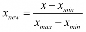
In words:

Normalized Measurement = (original measurement – minimum measurement value) divided by (maximum measurement value – minimum measurement value)

There numerous techniques for normalizing variables. A few are normalizing within a range of (-1 to 1), and mean normalization. And you might want to check out the coefficient of variation too.

Standardization

Standardization is a type of feature scaling and you may even hear it referred to as normalization. The formula below will transform your data so that the mean will be 0 and the standard deviation will be 1 (called a unit standard deviation).
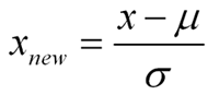
In words:

Standardized Measurement = (original measurement – mean of the variable) divided by (standard deviation of the variable)

When to Normalize? When to Standardize?

In many cases you can use normalization or standardization to scale your variables. However, if you have many outliers, normalization will not show outliers as well, because all data is scaled between two numbers (0,1).

On the other hand, standardization does not have any constraint on the resulting range of numbers. So, although in a normal distribution we would like the range of numbers to be between -3 and 3, they don’t have to be…so you will see outliers (such as values of say, -5 or 3.4, etc.) more easily.

Also, standardization makes it easy to see if a particular measurement is above or below the mean because negative numbers will be below the mean of 0 and positive numbers will be above the mean of 0.

And retaining the spread using standardization allows one to assign probabilities to measurements, and percentiles, while taking into account the spread of the data

References:

https://www.statisticshowto.datasciencecentral.com/normalized/

Standardization vs. normalization

Meta-Analysis and the Rewards of Persistence

Let’s say you would like to estimate the efficacy of a treatment or intervention but you don’t have the time, money, or other resources to design and implement an actual study. However, there are studies that have been performed by others. These studies can be reviewed and mined for information that will help you to investigate treatment effects. This is where a meta-analysis comes in handy.

In essence, a meta-analysis is an analysis of analyses. You can take the information obtained from a systematic review of the literature and obtain a pooled effect size and associated confidence interval for the treatment of interest.

Recently I worked on a rather large systematic review and meta-analysis of articles for a study on a therapeutic intervention for patients with dementia. The studies included a treatment group (sometimes more than one treatment group), and a control group, as well as baseline measurements, and one or more follow-up measurement times.

The outcomes of interest included continuous level measurements obtained from many different scales and survey instruments. Some scales/instruments were scored so that higher scores indicated improvement in functioning, whiles others were scored so that lower scores indicated improvement.

Deriving a pooled effect of treatment when there are numerous variations on measurement times, outcomes, and directions of the effects can be difficult. I needed to use special techniques to derive effect sizes and standard errors for each individual study and outcome. I ended up using standardized mean differences (SMD) which I could obtain from F-statistics, eta-squared values, or, if I was lucky, and the information was available, from the means and standard deviations for each group (treatment vs. control) at baseline and at the end of each study.

Oh, and many times, a single study would have numerous outcomes. What fun!

You’d think that computing the effect sizes for a conglomeration of studies with various designs, methods, and measurements would be the hard part…it wasn’t too bad once I figured it out. Here are some references and resources I used for computing the effects:

  • Morris, S. B. (2008). Estimating Effect Sizes From Pretest-Posttest-Control Group Designs. Organizational Research Methods, 11(2), 364-386.
  • Oooh, Check out this cool effect size calculator from Psychometrica!
  • The hard part was finding a way to compile the effect sizes into the pooled effect AND to design pretty forest plots that showed both (a) the individual studies and (b) the individual tests (outcomes) that were nested inside of each study.

    Many online resources and effect size calculators involved computing odds ratios from count data. But I had SMD’s from continuous data. Bummer…

    There are some very nice meta-analysis functions in Stata but I really struggled with getting the forest-plots to look pretty. I MUST HAVE PRETTY! And preferably without too much coding, gnashing of teeth and hair-pulling.

    There is a software, Comprehensive Meta-Analysis (CMA), which offers a free trial. And I tried the trial and it is very comprehensive! But again, I couldn’t get the forest plots to look the way I wanted them to look

    Finally, I came across an Excel add-on called MetaEasy, by Evangelos Kontopantelis and David Reeves.

    Excel? Really? Oh yes. And it was awesome. And FREE, my favorite four-letter word. The add-on was easy to install, the instructions were easy to follow. And the forest plots were very pretty.

    Here is a link which includes the download for MetaEasy, an instruction manual, and an Excel spreadsheet with example data.

    Here is a link to an example Excel spreadsheet I made using MetaEasy. In honor of the great Stan Lee I decided to compile it with studies of 11 of Mr. Lee’s superheroes with outcomes of improvement in mental health conditions based on the article, “10 Mental Health Problems Superheroes Suffer” I just made this up for demonstration purposes kiddos. So I don’t wish to discuss the details of who has what or why. Just have fun with it.

    I often find that if I keep digging I will hit treasure (not always, sometimes I puncture a sprinkler line). And I am happy to share this lovely golden nugget with you. Enjoy!

    Unique Identifiers. Gotta Have ‘Em!

    unique identifier portraits of people, all unique

    Before you use your data set you must be sure that each record in your data has a unique identifier (unique ID).

    Why? The best reason to assign unique ID’s is for tracking purposes. Trust me, you will run into a situation where a need to backtrack is necessary. There are many reasons, but here are two:

  • Perhaps a record is missing a value and you need to track the survey or find the information from a client or patient file.
  • Or, a study participant requests that their collected information be removed from a research study.
  • A unique identifier (ID) can be anything, as long as each record in your data set has a unique one of this thing. Typically a unique identifier is numeric, but it doesn’t have to be. If your data consists of survey respondents, you could use each respondents email (assuming respondents haven’t shared an email address!). Or maybe you’d like to use alpha-numeric ID’s. A way to determine what would work for your data is to ask, “What is the best unique information I have about the records in my data set?” You can then think about ways to fashion a nice unique ID for each record.

    Ok, you aren’t sure how to fashion your unique ID numbers for your records, or maybe you don’t really care about specifics of the unique ID, just that each record has one. Here are some tips on creating unique ID’s using SPSS software. I hope you find them useful!

    Let’s assume that your data is in a typical structure of a typical data set and you want to make a variable (a column) that gives each record (row) a unique identification number (ID).

    Here is some SPSS syntax to use to give a unique ID to each record in the dataset. The unique ID number will be the same as the row number of the record. SPSS refers to the row number as the “case number”.

    COMPUTE ID = $casenum.
    FORMAT ID (F8.0).
    EXECUTE.

    The FORMAT command says to give the variable you are creating (ID) for your unique ID number 8 digits, and 0 decimal places. ID’s don’t really need decimal places, but if you want to, just change the 0 to whatever number you want.

    Ok, easy peasy! But, what if you have a dataset in long format, with repeated measurements for some folks?

    I recently worked on a data set that included 3 years of data, but some participants were only in 1 year, some were in 2 years, and some others were in all 3 years.

    Every person had their own unique ID number, but the numbers were very long and it was hard to see the matches. And, I wanted to also see how many participants were in only 1 year, 2 years, or 3 years respectively.

    Another time you may want to do this is when you want to protect confidentiality of the participants. If the ID’s are traceable to participant records, such as patient numbers in hospital records or students in school records, or hey, the participant names are in the dataset! Then a new number that can’t be used to match to those records to outside sources should be created.

    So I needed to have unique ID numbers to replace the current ID numbers, and also needed to include a coding sequence for the possibility of a person having more than one measurement time. And, I wanted to know how many people were represented once, twice, or three times.

    I used these steps:

    1. First sort cases by the name or ID of the individuals.
    SORT CASES BY current_id(A).

    2. Under the “Data” pull down menu, choose “Identify Duplicate Cases”.

    — Define matching cases by: Move over the variable that is currently the ID into the box.

    — In the “Variables to Create” box, check the “Indicator of primary cases” box and specify “First Case in Each Group is primary” You will see a variable name such as “PrimaryFirst” in the box to the right. You can change the name to whatever you want.

    But I usually leave it as is.

    — Also check the box by “Sequential count of matching” this will count the number of instances each participant is represented.

    — Uncheck the “Move Matching cases to the top of the file” box. I don’t want to move anything around just yet.

    — But do check the “Display frequencies for created variables” box.

    3. Click “OK”.

    4. You should now have two variables at the right of the data set (a) PrimaryFirst and (b) MatchSequence. And you will have some output with frequencies of the matches etc.

    5. Now, we will use the two variables we created and some syntax to give the unique ID’s and they will be based on the case number variable. This syntax will give unique ID’s.

    BUT you will have some gaps in the numbering sequence due to the use of the case numbers to define the ID’s. For instance, you most likely won’t have ID that run 1, 2, 3, 4, 5, …. But they will be 1, 3, 4, 6, etc. Still UNIQUE though, and that is what we want!

    Here is the syntax to run:

    DO IF (PrimaryFirst EQ 1).
    COMPUTE ID = $casenum.
    else.
    COMPUTE ID = lag(ID).
    end if.
    EXECUTE.

    There should now be a variable called “ID” with a unique number given to each participant. You can now make a back-up of the file and don’t touch this one any more. Save the file also as a working file and then delete the “traceable” identifiers you don’t want to use from you working file.

    This working file will be used for all analyses, and sent to whomever needs to see it, but now you have, hopefully, protected some confidentiality of records.

    Also, you can use your new ID variable, and the MatchSequence variable as an index variable, if you need to transpose your data from long to wide.

    Now you’ll know who’s who and what’s what! 🙂

    Independent Samples t-test in Excel for Summary Data

    Mad Scientist Looking at a Beaker

    I recently had to run a series of independent samples t-tests on summary data, meaning I only had the group means, standard deviations, and sample sizes. There are online calculators available to do the job.

    But my client needed more information on what was going on behind the scenes of the calculations, and I needed a record of what I did. I looked for a way to run summary t-tests in SPSS and even R, and I couldn’t find a way.

    So I did what any gal with some stats knowledge and some coding experience would do.

    I made this calculator in Excel.

    Thanks to Todd Grande for the inspiration. I built my calculator based on his criteria. His video will walk you through it if you’d like to build one of your own. Or, you can just watch his video to see how it works. Enjoy!

    Control or Covariate?

    As is the case with many statistical concepts, one can find many terms for the same idea. And for many studies covariates and controls do the same work, but we call them different names according to how we use the variable.

    Technically, a covariate is a variable that is of no direct interest to the researcher, but one that may have an affect on the outcome (the dependent variable). Results of a study can be made more accurate by controlling for the variation in the covariate. So, a covariate is in fact, a type of control variable.

    Examples of a covariate may be the temperature in a room on a given day of an experiment or the BMI of an individual at the beginning of a weight loss program. Covariates are continuous variables and measured at a ratio or interval level.

    Technically, a control variable is a variable that is of no direct interest to the researcher….ok, it is more or less the same as a covariate, except, a control variable does not co-vary from record to record.

    This is the difference between covariates and controls in a study. For example, a covariate such as BMI can be different for each individual in the study, and it is theoretically able to have an infinite number of values depending on how many decimal places you want to count.

    A control variable is a nominal variable (not continuous) and although it has more than one value, the values are categorical and not infinite. Examples of a control variable could be the actual room number in which an experiment was conducted, or if an individual was underweight, normal weight, overweight, or obese.

    Recently, a client needed to include a measure of socio-economic status (SES) in her study and decided to use the variable of income. She wanted to know if she should define income as a covariate or a control in her analysis of variance (ANOVA). Of course I told her, as many statisticians do, that “It depends.”

    “On what?” you ask (and so did she). If we measure income in dollar amounts for each study participant, then we could use the information as a covariate, which would in turn make the ANOVA an analysis of co-variance (ANCOVA).

    However, if the variable was measured according to income group, such as $0 to $25,000; $25,001 to $50,000; $50,001 to $75,000; etc. then the variable would be a control variable and entered into the ANOVA as another independent grouped variable.

    So, both covariates and control variables can be considered “control variables”. The main difference is in the measurement level. If the variable is continuous, use it as a covariate. If you have categories, then you have an independent control variable. But don’t be surprised if you hear someone refer to a categorical control variable as a “covariate”. it is just the way of things in the wacky world of statistics.

    Propensity Scores vs. Regression Adjustment for Observational Studies

    Randomized controlled trials (RCTs) are considered the gold standard approach for estimating treatment effects. However, not all clinical research involves randomization of subjects into treatment and control groups. These studies are commonly referred to as non-experimental or observational studies. Some examples of non-experimental (observational) studies include:

  • Comparing a treatment group with a group of historical controls
  • Subjects pick the treatment they desire, hence, they self-select into a particular group
  • Subjects are compared on a variable that cannot be randomized, such as gender, race/ethnicity, drug use (yes/no)
  • Subjects are retrospectively pulled from a large dataset for review.
  • In observational studies, the treatment selection is influenced by the characteristics of subjects. Therefore, any differences between groups are not randomized out, and the baseline characteristics of the subjects could differ between treatment and control groups. In essence, the baseline characteristics systematically differ and we must find a way to account for these systematic baseline differences.

    Researchers often use regression adjustments to account for baseline differences between groups. A regression adjustment is made by using one or more (usually more) variables obtained at baseline as predictors, and one dependent variable of the treatment outcome. Using a regression adjustment to investigate baseline differences in observational studies has the following issues:

  • It is difficult to determine whether the model specification in a regression is the correct one to use. A researcher cannot reliably measure whether the variables he or she chooses are indeed the correct ones to use to control for the systematic baseline differences between groups. Model diagnostics such as the model R-squared of a multiple linear regression gives an indication of how well the predictors “predict” the outcome, but knowing how well a model fits as it relates to an outcome doesn’t tell us whether the model chosen actually included the predictors related to systematic baseline differences.
  • Using a regression model with the treatment as an outcome introduces researcher bias. This is because it can be very tempting for researchers to try different model specifications to get the model they desire. For instance, a researcher might, in good faith, start with a model that includes baseline variables that he or she believes are different between groups. Then, when the findings of the regression model indicate no significant effect on the outcome, or the model R-squared is too low, the researcher will change or add predictors to enhance the model. Not a good idea. And as noted above, it is very tempting to do.
  • Propensity scores, and matching subjects from each of the study groups using propensity scores, are constructed without taking the treatment outcome into consideration. The use of propensity scores keeps the researcher’s attention on baseline characteristics only. However, once the subjects are scored and matched (defined as balanced), a regression model can be analyzed to further adjust for any residual imbalance between the groups. So regression models still have their use! But they are used after the propensity scoring and matching.

    Propensity scores have the added benefit of allowing a researcher to see the actual amount of overlap, or lack of it, between treatment groups. After propensity scores are assigned to each individual in each group, then the researcher uses the scores to “match” pairs of subjects in the treatment with subjects in the control group. The easiest way to match is with a one-to-one match: one treatment subject to one control subject. But some, more-advanced matching techniques can match one-to-many.

    After matching, the researcher can see if there are many unmatched individuals left over (indicative of large differences in baseline characteristics between the groups). A large difference between groups might not just indicate that the treatment and control groups differed at baseline, but that the differences between groups might be too large to assess any meaning on the outcome of the intervention. After all, the reason for propensity score matching is to derive groups that simulate equal baseline characteristics. If they can’t be matched, they were just not similar. Hence, treatment efficacy cannot be derived or established.

    Here is a very simple example of the use of propensity scores and matching for a non-experimental study:

    A study is performed to assess the treatment effects of two analgesic drugs given to patients presenting to an emergency room with severe cluster headaches. The type of drug given, A or B, is decided upon various factors such as the time span of the current headache, frequency of headaches, age of the patient, and various comorbidities. Thus, the patients were not randomized into the two drug treaments.

    This non-randomization is also called “selection bias”. The clinician selected the treatment to give to each patient. If more than one clinician was involved in the decision making of treatment, we should control for this also! Perhaps some clinicians like one treatment over the other.

    The outcome is time to pain management. And looking at the data without any adjustment, Drug A appears to relive pain significantly faster than Drug B. But, maybe this is not the case. Something else could be at work here, or maybe there isn’t a difference between the drugs at all. Or maybe the patients in Group A (patients who took drug A) are much too different from the patients in Group B (patients who took Drug B) to make any assessment of efficacy.

    So, we will develop a propensity score for each patient based on the covariates we believe (or better, know from our knowledge and the literature). The propensity score, let’s call it Z, predicts how likely a person is to get Drug A.

  • We assume that the likelihood of a person receiving Drug A is very similar for all people with the same propensity score Z.
  • We then group people with similar propensity scores between the two groups of patients, such that patients with, say, Z = .30 in Group A are matched with patients with Z = .30 in Group B.

  • Then we can run tests on matched groups of patients to test treatment efficacy. With propensity score matching, we’ve removed some of the effects of baseline differences, and now we have something close to tiny RCT’s.

    Nothing is as good as the RCT, but I hope I’ve opened up your thinking a bit to the use of propensity scores in observational studies. There are many ways to score and match and analyze observational study groups. A good reference to start with is the article by Austin (2011) listed below. Rosenbaum and Rubin (1983) wrote the seminal work on propensity scores, but even I think it is a bit too theory heavy. But it is also listed in the references below if you are so inclined.

    Not everyone likes propensity scores for matching cases. The article by King and Nielsen (2016, also referenced below) presents some limitations in propensity score matching and some remedies for when many individual cases remain after the matching attempt.
    Stata has a function for tseffects for obtaining propensity scores, and the function of psmatch for propensity score matching. You can also run post-estimation regression with the functions.

    For R fans, here is a nice tutorial on propensity score matching. Not as nice as the Stata code, but hey, it’s free! http://pareonline.net/pdf/v19n18.pdf

    References

    Austin, Peter. (2011). An Introduction to Propensity Score Methods for Reducing the Effects of Confounding in Observational Studies. Multivariate behavioral research. 46. 399-424. 10.1080/00273171.2011.568786.

    R. Rosenbaum, Paul & B Rubin, David. (1983). The Central Role of the Propensity Score in Observational Studies for Causal Effects. Biometrika. 70. 41-55. 10.2307/2335942.

    Not everyone likes propensity scores for matching:
    Gary King and Richard Nielsen. Working Paper. “Why Propensity Scores Should Not Be Used for Matching”. Copy at http://j.mp/2ovYGsW

  • The Dissertation Proposal: Your Road Map to Success!

    The final dissertation defense, presented after all the data is analyzed and discussed, is the end of the journey for a Ph.D., and the road is never without speed bumps.  However, I find that too many candidates focus on the end of the journey and not the road map, the dissertation proposal.

    A properly planned proposal, typically the first three chapters of, (1) Introduction, (2) Literature Review, and (3) Methods, can make for a much more pleasant journey, or it can pave the way for detours and major hazards on the road to success.

    A dissertation proposal should be thought of as a contract between the candidate and committee.

    The proposal, especially the Methods chapter, details the specific steps in how the research will be conducted. Well, at least it details the plan. Things change, but it is good to have a detailed plan.

    I like to think of the Methods chapter as a recipe. Sure, maybe one will not be able to get vanilla extract and will need to substitute maple syrup. But in the end we are expecting a chocolate chip cookie, not just a generic dessert.

    I often see approved proposals, signed by the committee, with a data analysis section that simply, and inadequately, reads:

    The data will be analyzed using SPSS v.23 software. Descriptive statistics will include means and standard deviations of the study variables. The tests will include t-tests, ANOVA, and regression.

    Not defining in detail what data will be collected, how it will be collected, the variables that will be used for analysis, the coding of the variables for the analysis, and the specific statistical tests that will be used is a recipe for adding months, maybe years, to your journey.

    Why does this happen? I am sure there are many reasons. But often, especially in the online schools, committee members are overwhelmed with their workload and they do not take the time needed during the proposal phase to critically read and review a student’s proposal. Often, one committee member is designated as the methodologist or statistics expert, but they only know a bit about methodology, enough to be dangerous, and all other committee members follow his/her lead on the methodology. And too often, this results in the committee signing off on the proposal without a proper and thorough review.

    This of course, makes the dissertation candidate elated, because, well, the proposal was approved! GREAT NEWS!

    The happy (and unsuspecting) candidate then collects their data and then runs some numbers. But which of those statistical tests will answer the research questions? Maybe more than one will. Maybe none of them will. This is usually when a statistician gets a call to help, and sometimes there is not much that can be done. Then the methods must be re-worked to match the data collected…or it is just a wash. In either case, this delays the process, sometimes substantially.

    You should consider your Methods chapter as incomplete if it  does not include:

    • Specific details about the participants that will be included
    • The sampling plan
    • The operationalization (coding) of each variable that will be included in the tests
    • The hypotheses that will be tested to address the research questions
    • The specific statistical tests that will be used to test those hypotheses and specifications for those statistical models.
    • For more detailed studies, tables of variable levels and operationalizations, and the tests to be used, for each research question are a definite plus!

    A complete methods section with all of the details, signed by your committee and other powers that be (the AQR, IRB, etc.)  will keep these things from happening:

    • The new committee chair thinks you should concentrate on a larger or smaller group of participants. Perhaps they would like you to recruit only African American women instead of all African American students for your study.
    • A committee member read a journal article over Summer Break and now wants you to add social economic status to your study, but you’ve spent your Summer Break collecting data that only included gender, race/ethnicity, and marital status for your participants.
    • The committee doesn’t understand ANOVA and wants you to do 10 independent samples t-tests instead.

    Oh, I have dozens of stories…but you get the idea.

    My advice? Details, details, details!  Operationalize all of your variables, mention specific tests you will use. Detail, ad nauseam, every step in the process. Yes, it is a lot of work and most of it will involve statistical method and theory…

    But it will be worth it when you submit your completed dissertation with your Results chapter and Discussion to your committee or IRB and then they suggest (demand?) that another variable should be added, or that another test should be performed.

    With a detailed and signed proposal, you can take a deep breath, smile, point to your signed proposal (contract!) and say, “Wow, that is a great idea for my next study! But for now, let’s get this one finished according to our plan.”

    Your proposal is your contract. Make sure you’ve covered all of your bases and you’ll be glad you took the extra time in your travels on the road to success.

    Bridging the Gap: Choosing a Relevant Dissertation Topic

    Finding a suitable topic is the first of many challenges you will face in the dissertation process. Where do you even begin?

    The best place to start is with your own interests and the questions that have arisen for you over the course of your studies. You want to have familiarity with your subject matter. You will be working with it for quite a while!

    But what about that elusive gap in the literature? There are two valuable resources, (1) your committee and (2) the literature.

    Your Committee, Gotta Love ‘Em!

    Often a committee member or two will be actively involved in their own research and may be open to offering suggestions for further pursuing their research via your dissertation work.

    Although working on a committee member’s pet project sounds like an easy option, and it is in the beginning, it can become cumbersome for you as a researcher. A committee member with a vested interest in your success to enhance his/her research goals may be compelled to direct (meaning: control) your research more than you’d like. And often you will end up feeling like a research assistant who is only working to further the committee member’s goals and agenda.

    Having said this, many researchers do take on a committee member’s research and survive the process. But don’t say I didn’t warn you!

    The Literature, Your New Best Friend

    I cannot stress enough the need for a thorough literature review in your area of interest. Even if you have an idea of your topic, a literature review is necessary to:

    • Confirm interest in your planned topic, not just for yourself. Do others care? Is it considered important, even if by just a handful of people? Who are these people?
    • A literature review may also show you that work on your chosen topic has been exhausted and that the gap you were considering has been filled. No worries, it is better you know now than after you’ve written and submitted your proposal.
    • Inform you of the most recent findings and gaps in the research. The gaps can be found by reviewing the “implications for further study” in the Discussion sections of journal articles and other dissertations related to your planned topic. You could be just the person to address that need of further study, and in deciding to do so, BOOM, you have found your problem statement and literature gap!
    • A literature review is a possible first step in establishing relationships with renowned and current researchers in the field.
    • Why re-invent the wheel? Think about replicating a study, or gently tweaking a study, that you’ve found in your literature search. It is not plagiarism if you ask permission from the author(s) of the original study and if you note that you are replicating the study, with proper citations, in your work. Check the “suggestions for further research” sections of discussion chapters to see what the author thought were the next steps research. One of these “next steps” could be the basis of your study! For the most part, researchers love it when someone wants to replicate their work or use their instrumentation in a new study!

    Some General Advice

    • I mentioned earlier that you should be familiar with your topic because you will be working with it for quite a while. Also, your topic should be something that you are interested in. The time and money involved in the dissertation process is like remodeling a kitchen. It takes twice as long and costs twice as much as you think it will. So a topic that interests you will be much less mind numbing for you.
    • However, don’t study something that makes you emotionally upset (or joyful) or for which you have already formed a strong opinion. Bias is not a good thing in research and this is probably the best way to introduce it into a study. So avoid topics that are emotionally charged for you, no matter if the charge is positive or negative.
    • Parsimony is our friend. Only one gap needs to be addressed. So don’t attempt to fill in all the empty spaces. A big saying in my field is, “The best dissertation is a done dissertation.” Some of the best studies are simple and specific. And done!! Here is where the skills of a statistician who knows how to design a solid and robust research are needed. So keep my email and number handy and call when you are ready to design your study.
    • Don’t design your own survey instrumentation unless you absolutely on your life have too. There are all sorts of survey tools for any number of topics. So try to avoid designing your own unless you want to run a validation study for your tool inside of your actual study. Instead, search the literature for some tools that might work for you, and ask for permission from the designer of a tool to use it. The author’s email and place of work is usually right at the bottom of the first page of the journal article. Reach out. Most researchers love to see their instrumentation re-purposed because it adds to the validity of their tool.

    Next Steps?

      The second major challenge in the dissertation process is taking the research topic and designing a workable study around it. In a future post I will share some tips on how to turn your research topic into a research question.

      I am also planning a webinar to give you some tips and resources for refining your topic into a workable study! I’m still working on it, so keep in touch!

      In the meantime, check out a past webinar, Overview of Research Design, in the archives of the Omega Statistics channel on YouTube. And remember to sign up for the FREE literature review webinar in September, 2017. I look forward to seeing you there!

    Join the Stats for the Masses mailing list to receive the “Stats Grab Bag” email with useful resources and links relating to the work I do each week. I like to think of it as tidbits from practice. You’ll never know what you’ll get, but it could be just what you need!

    JOIN THE MAILING LIST


    Thank You - Watch Your Inbox For Our Next News Letter

    Accreditations and Memberships


    Murrieta Chamber Of Commerce Logo
    Better Business Bureau Logo
    American Statistical Association